Abstract

According to Dynamic Universe Model, our Universe is a Rotating Universe. In this model, electrons rotate about nucleus; Moons rotate about planets; Planets, asteroid and comets etc., rotate about stars; stars rotate about Galaxy center; Galaxies rotate about common center of local systems; and similarly Systems rotate in Ensembles, Aggregate, Conglomerations and Galaxy Clusters and so on and so forth. Galaxies coming near are Blue shifted and going away are red shifted. There are many blue shifted Galaxies in our universe. Here in this paper we will see different simulations to make such predictions from the output pictures formed from the Dynamic Universe model. There are some old and a few new simulations where different point masses are placed in different distances in a 3D Cartesian coordinate grid; and are allowed to move on universal gravitation force (UGF) acting on each mass at that instant of time at its position.  The output pictures depict the three dimensional orbit formations of point masses after some iterations.   In an orbit so formed, some Galaxies are coming near (Blue shifted) and some are going away (Red shifted). In this paper the simulations predicted the existence of a large number of Blue shifted Galaxies, in an expanding universe, in 2004 itself. Over 8,300 blue shifted galaxies have been discovered extending beyond the Local Group, was confirmed by Hubble Space Telescope (HST) observations in the year 2009. Thus Dynamic Universe model predictions came true.

Keywords

Rotating Universe; Dynamic Universe Model; Blue Shifted Galaxies; Hubble Space Telescope (HST); SITA Simulations   

Introduction

According to Dynamic Universe Model, our Universe is a Rotating Universe. In this model, electrons rotate about nucleus; Moons rotate about planets; Planets, asteroid and comets etc., rotate about stars; stars rotate about Galaxy center; Galaxies rotate about common center of local systems; and similarly Systems rotate in Ensembles, Aggregate, Conglomerations and Galaxy Clusters and so on and so forth. Galaxies coming near are Blue shifted and going away are red shifted. There are many blue shifted Galaxies in our universe. Both exist simultaneously unlike any expending universe model.

Dynamic Universe model is a singularity free tensor based math model. The tensors used are linear without using any differential or integral equations. Only one calculated output set of values exists.  Data means properties of each point mass like its three dimensional coordinates, velocities, accelerations and it’s mass. Newtonian two-body problem used differential equations. Einstein’s general relativity used tensors, which in turn unwrap into differential equations. Dynamic Universe Model uses tensors that give simple equations with interdependencies. Differential equations will not give unique solutions. Whereas Dynamic Universe Model gives a unique solution of positions, velocities and accelerations; for each point mass in the system for every instant of time. This new method of Mathematics in Dynamic Universe Model is different from all earlier methods of solving general N-body problem.

This universe exists now in the present state, it existed earlier, and it will continue to exist in future also in a similar way. All physical laws will work at any time and at any place. Evidences for the three dimensional rotations or the dynamism of the universe can be seen in the streaming motions of local group and local cluster. Here in this dynamic universe, both the red shifted and blue shifted Galaxies co-exist simultaneously.

How it all Started

Around 1543, Copernicus first proposed the planetary paths.  He pointed out that all Planets including the Earth moved around the SUN in De revolutionibus orbium coelestium.  This was a major step forward during that period.  Eventually, the circular planetary paths proposed by Copernicus were soon disproved by accurate astronomical observations [1].

The famous astronomer Tycho Brahe made accurate astronomical observations and after his death in 1601, Kepler worked on those observations.  Kepler published two laws in 1609 in Astronomia Nova – the first law talks about the elliptical path of planets around the Sun, where SUN is one of the two foci of the planetary path.  The second law states that the line joining the SUN and planets sweeps equal areas in equal intervals of time.  Kepler published a third law in Harmonice mundi in 1619 which states that the squares of the periods of planets are proportional to the cubes of the mean radii of their paths.  The third law was surprisingly accepted from the very first day it appeared in the journal. 

Kepler Orbit

Johannes Kepler’s laws of planetary motion around 1605, from astronomical tables detailing the movements of the visible planets. Kepler's First Law is:

"The orbit of every planet is an ellipse with the sun at a focus."

The mathematics of ellipses is thus the mathematics of Kepler orbits, later expanded to include parabolas and hyperbolas.

Sir Isaac Newton’s Law of Universal Gravitation (1687)

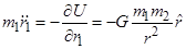
Every point mass attracts every other point mass by a force pointing along the line intersecting both points. The force is proportional to the product of the two masses and inversely proportional to the square of the distance between the point masses:

Where:

F is the magnitude of the gravitational force between the two point masses,

G is the gravitational constant,

m₁ is the mass of the first point mass,

m₂ is the mass of the second point mass,

r is the distance between the two point masses.

Newton: Two-body Problem

In mechanics, the two body problem is a special case of the n-body problem with a closed form solution.  This problem was first solved in 1687 by Sir Isaac Newton [2] who showed that the orbit of one body about another body was either an ellipse, a parabola, or a hyperbola, and that the center of the mass of the system moved with constant velocity.  If the common center of mass of the two bodies is considered to be at rest, each body travels along a conic section which has a focus at the common center of the mass of the system.  If the two bodies are bound together, both of them will move in elliptical paths.  If the two bodies are moving apart, they will move in either parabolic or hyperbolic paths. The two-body problem is the case that there are only two point masses (or homogeneous spheres); If the two point masses  (r₁, m₁) and (r₂, m₂) having  masses m₁ and m₂ and the position vectors r₁ and r₂ relative  to a point with respect to their common centre of mass, the equations of motion for the two mass points are :

Where is the distance between the bodies; U (|r₁ − r₂|) is the potential energy and

is the unit vector pointing from body 2 to body 1. The acceleration experienced by each of the particles can be written in terms of the differential equation

          (1)   

Where µ = G·M;  M being the mass of the body causing the acceleration (i.e m₁ or the acceleration on body 2). The mathematical solution of the differential equation (1) above will be: Like for the movement under any central force, i.e. a force aligned with  the specific relative angular momentum

 stays constant:

                                           

                                                                         

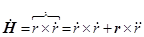
                                                                               = 0 + 0 = 0

Sir Isaac Newton published the Principia in 1687. Halley played an important role in getting Principia published.  Sir Isaac discussed the inverse square law of force and solved it in Prop. 1-17, 57-60 in Book I [31].  In Book I, Newton argued that orbits are elliptical, parabolic or hyperbolic due to inverse square law.  Newton also deduced Kepler’s third law in the Principia. 

Halley ’s Comet

Halley adopted Newton’s method to compute the almost parabolic orbits of a number of comets.  He was able to prove that the comet which appeared in the year 1537, 1607 and 1682 (which was previously thought to be three different comets) was only one comet which had followed the same orbit.  He was later able to identify it with the one which appeared in 1456 and 1378.  He was able to compute the elliptical orbit for the comet, and he noticed that Jupiter and Saturn were perturbing the orbit slightly between each return of the comet. Taking the perturbations into account, Halley predicted that the comet would return and reach perihelion (the point nearest the Sun) and it would appear again on 13 April, 1759 plus or one month.  The comet actually appeared in 1759 reaching the perihelion on 12 March.

The purpose here is simply to point to the complex formal descriptions of the dynamic relationships in each case. Note that simpler satisfactory solutions may be found in each case if particular constraints are allowed. Many mathematicians have given considerable attention to the solution of the equations of motions for N gravitationally interacting bodies.

Dynamic Universe Model: Blue and Red Shifted Galaxies

In this Dynamic Universe Model – Galaxies in a cluster are rotating and revolving. Depending on the position of observer’s position relative to the set of galaxies, some may appear to move away, and others may appear to come near. The observer may also be residing in another solar system, revolving around the center of Milky Way in a local group. He is observing the galaxies outside. Many times he can observe only the coming near or going away component of the light ray called Hubble components. The other direction cosines of the movement may not be possible to measure exactly in many cases. It is an immensely complicated problem to untangle the two and pin point the cause of non–Hubble velocities. This question was discussed by JV. Narlikar in (1983) see the ref [3]. ’Nearby Galaxies Atlas’ published by Tully and Fischer contains detailed maps and distribution of speeds of Galaxies in the relatively local region.[4] The multi component model used by them uses the method of least squares. Hence we can say that Galactic velocities are possible in all the directions.

Let’s start with an analogy. Imagine one person standing near a giant wheel in a children’s park. When the wheel is rotating and the person is standing on the axis of wheel, he will see all the buckets moving and none come near or go away. When the person is standing in the plane of giant wheel rotation, he will see some buckets come near at the top and some go away at the bottom. All the other buckets will have some upward motion or downward motion, combined with either coming near or going away. Depending on the person’s position relative to the plane of rotation, the overall effect of buckets going away or coming near will vary.  It is peculiar motion of buckets in the plane. Peculiar motion can be in any direction in the three dimensional sphere from the center.

Now, let us imagine 10 such giant wheels rotating about each other and such 6 sets of (10 giant wheels in each set, of course both 6 & 10 are arbitrary numbers) rotating giant wheels rotating about each other all in different planes. These giant wheels, can be rotating about each other, when there no huge central mass. No problem.  All depends on their positions and instantaneous velocities. Imagine yourself in one bucket and observing a distant bucket in different giant wheel with a telescope. You can see only observed bucket going away or coming near. That observed giant wheel will have a bigger velocity component of going away super imposed on its coming near component of velocity in the observed motion of bucket. In a 3 dimensional space there are many directions. Some can come near purely towards you (Blue-shift). All the others will have some component of going away (red-shift). This red-shift component is readily measured in the case of a Galaxy, which is having its own peculiar motion. Here one can visualize why Blue-shifted galaxies (or the buckets in our analogy without any outgoing velocity component) are less.

Present-day Peculiar Motions of Galaxies, Hubble Flow, Distant Red-Shifted Galaxies

‘Peculiar motions’ of Galaxies is the thing predicted by Dynamic Universe Model theoretically, whereas a Bigbang based cosmology predicts only radially outward motion from earth or red-shifted Galaxies and no blue-shifted Galaxies at all.

Local group of Galaxies are present up to a distance of 3.6 MPC. From that point onwards, we will find red-shifted Galaxies. I don’t know where actually Hubble flow starts. But I think that is the distance of 3.6 MPC where so called Hubble-flow starts. If the Hubble flow does not start here, why do red-shifted galaxies appear from this distance onwards?  If the Hubble–flow is such strong, why would it leave some 8300 blue-shifted Galaxies? Anybody can see the updated list of Blue shifted Galaxies in the NED. (NASA/IPAC EXTRAGALACTIC DATABASE) by JPL anybody can get the exact number of Blue shifted Galaxies by Hubble space telescope to the present date & time. (If you need any assistance in searching NED, please contact the author) As on 4th April 2012 at 1210 hrs Indian time, it is 7306 Blue-shifted galaxies. But presently this search gives 8300. Some current active research and discussions can be found in physics forums by searching ‘blue-shifted-galaxies-there-are-more’.

We are discussing ‘Hubble flow’ as some unknown force pulling away all the galaxies to cause the expansion of universe. But in reality it is the going away component of ‘peculiar motion’ of that particular Galaxy. That Galaxy may be moving in any direction in reality. Each Galaxy move independently, with the gravitational force of its Local group, clusters etc. There is no separate Hubble force to cause a separate Hubble flow…

Different estimates of distances of Blue-shifted Galaxies especially in Virgo Cluster are varying. There are about 3000 blue-shifted Galaxies in Virgo cluster. Some estimate for the most distant Blue-shifted Galaxy in Virgo cluster may go as high as 40 MPC, and other estimate go as low as 17 MPC. I don’t know whom to believe. Here distance estimate is not dependent on Red / Blue shift, but dependent on various other methods. Here probably the distance and red shift proportionality is not working. So we can see that blue shifted Galaxies are not confining to earlier thinking of 3.6 MPC distances. Here, the estimated distance is not depending on Red / Blue shift, but on various other methods.  Accurate measurement of distances after 40 MPC depends mostly on red-shift only. There is a hope to find an accurate estimate of distance, if type 1a Supernova standard candle is observed in a Galaxy. When we are estimating the distance with red-shift, finding far off blue-shifted Galaxies is not possible.

All these findings are from some recent times only. Hence nothing can be said about the peculiar motions of blue shifted Galaxies. All these velocities are at present radial velocities only.  A lot of work is to be done in these lines.

In general, whether the Source is emitting radiation in Infrared (Microwave or some lover frequencies) region or lower, or the Source is in Ultra violet (X-rays or higher) frequency region, we take the source as red-shifted only. The sources which emit only X-rays were taken as red-shifted, though by definition, X-rays are blue-shifted, due to their higher frequency. Even if the source is emitting a single frequency radiation, we find it is only red-shifted.

History of Blue Shifted Galaxies ---Let’s Start with Charles Messier

After 1922 Hubble published a series of papers in Astrophysical Journal describing various Galaxies and their red shifts / blue shifts. Using the new 100 inch Mt. Wilson telescope, Edwin Hubble was able to resolve the outer parts of some spiral nebulae as collections of individual stars and identified some Cepheid variables, thus allowing him to estimate the distance to the nebulae: they were far too distant to be part of the Milky Way. In the Ref. [5, 6]  one can find more detailed analysis of this issue. And later using 200 inch Mt Palomar telescope Hubble could refine his search. In 1936 Hubble produced a classification system for galaxies that is used to this day, the Hubble sequence.

In the 1970s it was discovered in Vera Rubin's study of the rotation speed of gas in galaxies that the total visible mass (from the stars and gas) does not properly account for the speed of the rotating gas. This galaxy rotation problem is thought to be explained by the presence of large quantities of unseen dark matter. This dark matter question was discussed by Vera Rubin, see the Ref. [1, 2].

In fact there are millions of Blue shifted Galaxies not just 8300 found from 2009 by Hubble space telescope. ‘Beginning in the 1990s, the Hubble Space Telescope yielded improved observations. Among other things, Go to ADS search page try searching title and abstract with keywords “Blue shifted quasars”.  If you search with “and”s ie., ‘Blue and Shifted and Galaxies” [use “and” option not with “or”option] you will find 248 papers in ADS search. I did not go through all of them.  it established that the missing dark matter in our galaxy cannot solely consist of inherently faint and small stars. One can find more detailed analysis of this issue in the published ltarature on Hubble Deep Field, They gave an extremely long exposure of a relatively empty part of the sky, provided evidence that there are about 125 billion (1.25×10¹¹) galaxies in the universe. Further details can be found at ref [5]. Improved technology in detecting the spectra invisible to humans (radio telescopes, infrared cameras, and x-ray telescopes) allow detection of other galaxies that are not detected by Hubble. Particularly, galaxy surveys in the Zone of Avoidance (the region of the sky blocked by the Milky Way) have revealed a number of new galaxies. In the Ref. [7] one can find more detailed analysis of this issue.

Hubble Space Telescope’s improved observational capabilities resolved as many as 8300 galaxies as Blue shifted till today which will discuss later in this paper.

Prediction of Blue Shifted Galaxies

In this paper, different sets of point masses were taken at different 3 dimensional positions at different distances. These masses were allowed to move according to the universal gravitation force (UGF) acting on each mass at that instant of time at its position. In other words each point mass is under the continuous and Dynamical influence of all the other masses. For any N-body problem calculations, the more accurate our input data the better will be the calculated results; one should take extreme care, while collecting the input data. One may think that ‘these are simulations of the Universe, taking 133 bodies is too less.’ But all these masses are not same, some are star masses, some are Galaxy masses some clusters of Galaxies situated at their appropriate distances. All these positions are for their gravitational centres. The results of these simulation calculations are taken here. 

Original submission of this paper “No Big bang and GR: proves DUMAS! (Dynamic Universe Model of cosmology: A computer Simulation)”,  DSR894 was done on 2nd April 2004 to Physical Review D.  Currently, this paper is being thoroughly revised and resubmitted. [8], Here in these simulations the universe is assumed to be heterogeneous and anisotropic. From the output data graphs and pictures are formed from this Model.   These pictures show from the random starting points to final stabilized orbits of the point masses involved.   Because of this dynamism built in the model, the universe does not collapse into a lump (due to Newtonian gravitational static forces). This Model depicts the three dimensional orbit formations of involved masses or celestial bodies like in our present universe. From the resulting graphs one can see the orbit formations of the point masses, which were positioned randomly at the start. An orbit formation means that some Galaxies are coming near (Blue shifted) and some are going away (Red shifted) relative to an observer’s viewpoint.

New simulations were conducted. The resulting data graphs of these simulations with different kinds of input data are shown in this paper in the later parts.

In all these simulations, all point masses will have different distances, masses.

- Simulation 1: All point masses are Galaxies

- Simulation 2: All point masses are Globular Clusters

- Simulation 3: Globular Clusters 34 Galaxies 33 aggregates 33 conglomerations 33

- Simulation 4: Small star systems 10 Globular Clusters 100 Galaxies 8 aggregates 8 conglomerations 7

The problem with such simulations is the overwhelmingly large amounts of output data. Each simulation gives 3 dimensional vector data of accelerations, velocities, positions for every point mass in every iteration in addition to many types of derived data. A minimum of 133 x 18 dataset of 16 decimal digits will be generated in every iteration.  It is data and data everywhere. It is a huge data mine indeed. 

A point to be noted here is that the Dynamic Universe Model never reduces to General relativity on any condition. It uses a different type of mathematics based on Newtonian physics. This mathematics used here is simple and straightforward. As there are no differential equations present in Dynamic Universe Model, the set of equations give single solution in x y z Cartesian coordinates for every point mass for every time step. All the mathematics and the Excel based software details are explained in the three books published by the author[9, 10, 11] In the first book, the solution to N-body problem-called Dynamic Universe Model (SITA) is presented; which is singularity-free, inter-body collision free and dynamically stable. The Basic Theory of Dynamic Universe Model published in 2010 [9]. The second book in the series describes the SITA software in EXCEL emphasizing the singularity free portions. This book written in 2011 [10] explains more than 21,000 different equations. The third book describes the SITA software in EXCEL in the accompanying CD / DVD emphasizing mainly HANDS ON usage of a simplified version in an easy way. The third book is a simplified version and contains explanation for 3000 equations instead of earlier 21000 and this book also was written in 2011[11]. Some of the other papers published by the author are available at refs. [6, 8,12, 13, 14, 15, 16, 17].

SITA solution can be used in many places like presently unsolved applications like Pioneer anomaly at the Solar system level, Missing mass due to Star circular velocities and Galaxy disk formation at Galaxy level etc. Here we are using it for prediction of blue shifted Galaxies.

Co-Existence of Red and Blue Shifted Galaxies

These simulations of Dynamic Universe Model predicted the existence of the large number of Blue shifted Galaxies in 2004, ie., more than about 35 ~ 40 Blue shifted Galaxies known at the time of Astronomer Edwin Hubble in 1930s. See the ref [6]. The far greater numbers of Blue shifted galaxies was confirmed by the Hubble Space Telescope (HST) observations in the year 2009. Today the known number of Blue shifted Galaxies is more than 8300 scattered all over the sky and the number is increasing day by day. This is a greater number compared to 30-40 Blue shifted galaxies earlier. 

In addition the author presumes that there is a greater probability that the Quasars, UV Galaxies, X-ray, γ- Ray sources and other Blue Galaxies etc., are also Blue shifted Galaxies. Another assumption can be made about images of Galaxies. A safe assumption can be… out of a 930,000 Galaxy spectra in the SDSS database, about 40% are images for Galaxies; that leaves about 558,000 as Galaxies.  If both the assumptions are correct, then there are 120,000 Quasars, 50,000 brotherhood of (X-ray, γ-ray, Blue Galaxies etc.,) of quasars, 8300 blue shifted galaxies. That is about 32% of available Galaxy count are Blue shifted. And if we don’t assume any images and assume about Quasars etc only, then it will be about 20% are Blue shifted Galaxies. 

Ours is not a steady state universe in the sense, it does not require matter generation through empty spaces. No starting point of time is required. Time and spatial coordinates can be chosen as required.  No imaginary time, perpendicular to normal time axis, is required. No baby universes, black holes or warm holes were built in.

This approach solves many prevalent mysteries like Galaxy disk formation, Missing mass problem in Galaxy–star circular velocities, Pioneer anomaly, etc. Live New horizons satellite trajectory predictions are very accurate and are comparable to their ephemeris.

This universe exists now in the present state, it existed earlier, and it will continue to exist in future also in a similar way. All physical laws will work at any time and at any place. Evidences for the three dimensional rotations or the dynamism of the universe can be seen in the streaming motions of local group and local cluster. Here in this dynamic universe, both the red shifted and blue shifted Galaxies co-exist simultaneously.

Types of Blue Galaxies Whose Radiation is found in UV and above Frequencies ( Blue Shifted Galaxies)

There are many types of Galaxies. Many of them are into blue shift. Some types like Starburst, AGNs, UV and Gamma ray can be a safe bet for blue shifted Galaxy candidates. Classifying the starburst / AGN category itself isn't easy since starburst galaxies don't represent a specific type in themselves. Blue shifted Galaxies can occur in disk galaxies, spherical in any other shapes. And especially in irregular galaxies which often exhibit knots of starburst, often spread throughout the irregular galaxy are possible Blue shifted Galaxies. Let’s see various possible Blue shifted Galaxies below:

Blue compact galaxies (BCGs), Active galactic nucleus (AGN), Radio-quiet AGN, Seyfert galaxies, Radio-quiet quasars/QSOs, 'Quasar 2s', Radio-loud quasars, Radio-quit quasars, 'Blazars' (BL Lac objects and OVV quasars), Radio galaxies, Blue compact dwarf galaxies(BCD galaxy), Pea galaxy (Pea galaxies), Luminous infrared galaxies (LIRGs), Ultra-luminous Infrared Galaxies (ULIRGs), and Hyperluminous Infrared galaxies (HLIRGs).

Evidences for AGNs and Quasars are Blue Shifted Galaxies--- Present Day Concept of Quasars

Quasars are among the most luminous, powerful and energetic objects known in the universe and can emit up to a thousand times the energy output of the Milky Way [2]. Quasars have all the same properties as active galaxies and AGNs, but are more powerful. The radiation emitted by quasars is across the spectrum, almost equally, from X-rays to the far-infrared with a peak in the ultraviolet-optical bands, with some quasars also being strong sources of radio emission and of gamma-rays.  Additionally Quasars can be detected over the entire observable electromagnetic   spectrum including radio, infrared, optical, ultraviolet, X-ray and even gamma rays. Their radiation is partially 'non-thermal' i.e., not due to a black body. In early optical images, quasars looked like single points of light (i.e., point sources), indistinguishable from stars, except for their peculiar spectra. With infrared telescopes and the Hubble Space Telescope, the "host galaxies" surrounding the quasars have been identified in some cases. These galaxies are normally too dim to be seen against the glare of the quasar, except with these special techniques. Most quasars cannot be seen with small telescopes, but 3C 273, with an average apparent magnitude of 12.9, is an exception. At a distance of 2.44 billion light-years, it is one of the most distant objects directly observable with amateur equipment. In Part 4, this quasar 3C 273 was shown to have a blue shift of (0.143122).

About 8% to 15% of Quasars have jets with lengths of millions of light years. These jets carry significant amounts of energy in the form of high-energy particle that move with speeds close to the speed of light consisting of either electrons and protons or electrons and positrons.

The Active Galactic Nuclei popularly known as AGNs and Quasars are Blue shifted Galaxies. Let us discuss about the quasars and AGNs in a next paper. One can see [15, 18, 19] for additional information.

Dynamic Universe Model as an Universe Model

Dynamic universe model is different from Newtonian static model, Einstein’s Special & General theories of Relativity, Hoyle’s Steady state theory, MOND, M-theory & String theories or any of the Unified field theories. It is basically computationally intensive real observational data based theoretical system. It is based on non-uniform densities of matter distribution in space. There is no space time continuum. It uses the fact that mass of moon is different to that of a Galaxy. No negative time. No singularity of any kind. No divide by zero error in any computation/ calculation till today.  No black holes, No Bigbang or no many minute Bigbangs. All real numbers are used with no imaginary number. Geometry is in Euclidian space. Some of its earlier results are non-collapsing, non-symmetric mass distributions. It proves that there is no missing mass in Galaxy due to circular velocity curves. Today it tries to solve the Pioneer anomaly. It is single closed Universe model.

Our universe is not a Newtonian type static universe. There is no Big bang singularity, so “What happened before Big bang?” question does not arise. Ours is neither an expanding nor contracting universe.  It is not infinite but it is a closed finite universe.  Our universe is neither isotropic nor homogeneous. It is LUMPY. But it is not empty. It may not hold an infinite sink at the infinity to hold all the energy that is escaped. This is closed universe and no energy will go out of it. Ours is not a steady state universe in the sense, it does not require matter generation through empty spaces. No starting point of time is required. Time and spatial coordinates can be chosen as required.  No imaginary time, perpendicular to normal time axis, is required. No baby universes, black holes or warm holes were built in.

This approach solves many prevalent mysteries like Galaxy disk formation, Missing mass problem in Galaxy–star circular velocities, Pioneer anomaly, etc. Live New horizons satellite trajectory predictions are very accurate and are comparable to their ephemeris.

This universe exists now in the present state, it existed earlier, and it will continue to exist in future also in a similar way. All physical laws will work at any time and at any place. Evidences for the three dimensional rotations or the dynamism of the universe can be seen in the streaming motions of local group and local cluster. Here in this dynamic universe, both the red shifted and blue shifted Galaxies co-exist simultaneously.

Dynamic universe Model: General Introduction

Dynamic Universe Model of Cosmology is a singularity free N-body solution. It uses Newton’s law of Gravitation without any modification. The initial coordinates of each mass with initial velocities are to be given as input. It finds coordinates, velocities and accelerations of each mass UNIQUELY after every time-step. Here the solution is based on tensors instead of usual differential and integral equations. This solution is stable, don’t diverge, did not give any singularity or divided by zero errors during the last 18 years in solving various physical problems. With this model, it was found with uniform mass distribution in space, the masses will colloid but no singularities. With non-uniform mass densities, the masses trend to rotate about each other after some time-steps and they don’t colloid. SITA (Simulation of Inter-intra-Galaxy Tautness and Attraction forces) is a simple computer implementable solution of Dynamic Universe Model and other solutions were possible. An arbitrary number of 133 masses were taken in SITA simulations using the same framework in solving various problems.

Euclidian space, real number based coordinate axes, no space-time continuum, non-uniform mass distribution, no imaginary dimensions, simple Engineering achievable physics are basis. This SITA simulation is a calculation method using a math framework and where we input values of masses, initial distances and velocities to get various results. Based on these it achieves a non-collapsing and dynamically balanced set of masses i.e. a universe model without Bigbang & Black-hole singularities. This approach solves many prevalent mysteries like Galaxy disk formation, Missing mass problem in Galaxy –star circular velocities, Pioneer anomaly, New Horizons trajectory calculations and prediction, Blue shifted Galaxies in Expanding Universe...  etc. With this Dynamic Universe model, we show Newtonian physics is sufficient for explaining most of the cosmological phenomena.

In Dynamic Universe Model, there are no singularities and no collisions if we use heterogeneous mass distributions. When homogeneous mass distributions are used, there are collisions but no singularities. Resultant Universal Gravitational Force is calculated for each body for every timestep in all the three dimensions. Conservation of energy, moment etc, were taken into consideration as shown in the Mathematical formulation. Using exactly same setup of mathematics and SITA algorithm and same number of 133 masses, all the results are derived, in the last 18 years.

Dynamic Universe Model is a mathematical framework of cosmology of N-body simulations, based on classical Physics. Here in Dynamic Universe Model all bodies move and keep themselves in dynamic equilibrium with all other bodies depending on their present positions, velocities and masses. This Dynamic Universe Model is a finite and closed universe model. Here we first theoretically find the Universal gravitational force (here after let us call this as UGF) on each body/ particle in the mathematical formulation section in this book. Then we calculate the resultant UGF vector for each body/ particle on that body at that instant at that position using computer based Simulation of Inter-intra-Galaxy Tautness and Attraction forces  (here after let us call this as SITA simulations) which simulate Dynamic universe model. Basically SITA is a calculation method where we can use a calculator or computer; real observational data based theoretical simulation system. Initially 133 masses were used in SITA about 18 years back, after theoretical formulation of Dynamic universe model. Using higher number of masses is difficult to handle, which was a limitation of 386 and 486 PCs available at time in the market. I did not change the number of masses until now due to two reasons. Firstly getting higher order computers is difficult for my purse as well as additional programming will also be required. Secondly, I want to see and obtain the different results from the same SITA and math framework.  There are many references by the author presenting papers in many parts of the world.

Let’s start with Charles Messier

Charles Messier started the galaxies era. Astronomer Hubble found the blue shift of Andromeda. The Quasars are Blue shifted Galaxies. Finally Blue shifted galaxies found by Hubble Space Telescope. Let’s see briefly what happened in between.

Charles Messier was one of the first discoverers of the nebulae and the galaxies. He compiled a catalog of 109 brightest nebulae in about 1780 onwards. In around 1850s,William Herschel compiled a larger catalog of 5000 objects. Lord Rosse constructed a new telescope and was able to distinguish between elliptical and spiral nebulae.

Galaxies were not recognized as a distinct kind of nebular object until the late 19th century, when visual spectroscopy (Huggins) of the Andromeda spiral (M31) showed a continuous spectrum.  Distinct structure was reported by William Parsons, 3rd Earl of Rosse known as lord Rosse, whose 72-inch speculum-metal reflector showed clear spiral features in some bright nebulae such as M33, M51, and M101.

In 1912, Vesto Slipher made spectrographic studies of the brightest spiral nebulae to determine if they were made from chemicals that would be expected in a planetary system. However, Slipher discovered that the spiral nebulae had high red shifts, indicating that they were moving away at rate higher than the Milky Way's escape velocity. Thus they were not gravitationally bound to the Milky Way, and were unlikely to be a part of the Milky Way.

In 1917, Heber Curtis had observed a nova S Andromedae within the "Great Andromeda Nebula" (as the Andromeda Galaxy, Messier object M31, was known). Searching the photographic record, he found 11 more novae. Curtis noticed that these novae were, on average, 10 magnitudes fainter than those that occurred within our galaxy. As a result, he was able to come up with a distance estimate of 150,000 parsecs. He became a proponent of the so-called "island universes" hypothesis, which holds that spiral nebulae are actually independent galaxies. In 1922, astronomer Ernst Öpik gave a distance determination, which supported the theory that the Andromeda Nebula is indeed a distant extra-galactic object.

After 1922 Hubble published a series of papers in Astrophysical Journal describing various Galaxies and their red shifts / blue shifts. Using the new 100 inch Mt. Wilson  telescope, Edwin Hubble was able to resolve the outer parts of some spiral nebulae as collections of individual stars and identified some Cepheid variables, thus allowing him to estimate the distance to the nebulae: they were far too distant to be part of the Milky Way. And later using 200 inch Mt Palomar telescope Hubble could refine his search. In 1936 Hubble produced a classification system for galaxies that is used to this day, the Hubble sequence.

In the 1970s it was discovered in Vera Rubin's study of the rotation speed of gas in galaxies that the total visible mass (from the stars and gas) does not properly account for the speed of the rotating gas. This galaxy rotation problem is thought to be explained by the presence of large quantities of unseen  dark matter [1,2]

From 1970 to 2006 there were as many as 248 papers published in various journals describing the Blue shift properties of Quasars [4].

Beginning in the 1990s, the Hubble Space Telescope yielded improved observations. Among other things, it established that the missing dark matter in our galaxy cannot solely consist of inherently faint and small stars. [13]The Hubble Deep Field, an extremely long exposure of a relatively empty part of the sky, provided evidence that there are about 125 billion (1.25×10¹¹) galaxies in the universe. [5]Improved technology in detecting the spectra invisible to humans (radio telescopes, infrared cameras, and x-ray telescopes) allow detection of other galaxies that are not detected by Hubble. Particularly, galaxy surveys in the Zone of Avoidance (the region of the sky blocked by the Milky Way) have revealed a number of new galaxies [7].

Hubble Space Telescope’s improved observational capabilities resolved as many as 7300 galaxies as Blue shifted till today which will discuss later in this book. See Wikipedia for some further details [12].

I did not touch a lot many historical events.

Dynamic Universe Model – Introduction

Dynamic Universe Model    is a totally non-general relativistic algorithm. Here in no way GR effects are taken into consideration and this model doesn’t reduce to GR on any condition. No space-time continuum. In this Dynamic Universe Model all the bodies in Universe are assumed to be dynamically moving.

This Dynamic Universe Model is a set of MATH equations for solving N-body problem. With SITA software it behaves like a hand held Calculator. SITA software in a PC will work like a Calculator for solving a typical N-body problem. Using the same set of equations one can give different initial values numerically to solve various different problems at different scales. These initial values (the Cartesian x, y, z positions and velocities & time step) are different for different applications. The distant Galaxies or distant local systems can be assumed as point masses with mass at their center of Gravity. That way the number of masses can be as low as 133 and otherwise this simulation can be done on higher number of masses also. The main concept is as follows:

There are many secrets embedded in the Universe that are still unexplored. A simple uniform law may not explain all the peculiarities in the ever changing Dynamic universe. In fact, the uniform density is not observable at any scale because of large Voids and Great walls present in the Universe. Earth is not the center of universe. Our universe is finite. The view from earth is not being uniform in all the directions.

This universe is now in the present state, as existed earlier and will continue to exist in the same way. This is something like Hoyle’s Steady state model philosophy [7] but without creation of matter. PCP (Perfect Cosmological Principle) was not considered true here as in steady state universe. We need not assume any homogeneity and isotropy here at any point of time. Matter need not be created to keep the density constant. Here Bigbang like creation of matter is also not required. Blue shifted galaxies also exist along with red shifted ones. No dark energy and dark matter is required to explain physical phenomena here. Here in this model the present measured CMB is from stars, galaxies and other astronomical bodies. This Dynamic Universe Model is a closed universe model.

Our Universe is not empty. For example De Sitter’s universe model explains everything but his Universe has no matter in it [6]. It may not hold a sink to hold all the energy that is escaped from the universe at infinity.[ref Einstein] It is a finite and closed universe. Absolute Rest frame of reference is not necessary. The time and space coordinates can be chosen as required. Dynamic Universe Model is different from Fritz Zwicky’s tired light theory as light does not loose energy here[8].   Gravitational red shift is present here.

Dynamic Universe Model gives a daring new approach. It is different from Newtonian static model and Olber’s paradox [14]. Here masses don’t collapse due to self-gravitation and even though the masses are finite in number, they balance with each other dynamically and expanding. There is no space-time continuum. Hawking and Penrose[15,18] (1969, 1996) in their singularity theorem said that ‘In an Isotropic and homogeneous expanding universe, there must be a Big bang singularity sometime in the past according to General theory of relativity ’. Since Isotropy and Homogeneity is not an assumption in Dynamic Universe Model, singularity theorem is not applicable here and Hawking’s Imaginary time axis perpendicular to time axis is not required. No baby universes, Blackhole or wormhole singularity [19] is built in. No Bigbang singularity [9 ] as in Friedmann-Robertson-Walker models. JV Narlikars’ many mini Bigbangs are also not present here[10]. Also this Dynamic Universe Model is poles apart from, M-theory & String theories or any of the Unified field theories. The basic problem in all these models, including String theory[11] and M-theory[16]  is that the matter density is significantly low and they push Bigbang singularity into some other dimensions.

There is a fundamental difference between galaxies / systems of galaxies and systems that normally use statistical mechanics, such as molecules of air in a box, the similarly charged particles repel each other but in gravitation we have not yet experienced any repulsive forces. Only attraction forces were seen in Newtonian and Bigbang based cosmologies. (See for ref: Binny and Tremaine 1987[3]). But here in Dynamic Universe Model masses when distributed heterogeneously experience repulsive forces as well as attractive forces due to the total resulting UGF: the Universal Gravitational Force acting on the particular mass. Einstein’s cosmological constant l[17] to introduce repulsive forces at large scales like inter galactic distances (as also in MOND), is not required here.

In this Dynamic Universe Model, bodies move in dynamic equilibrium to compensate for the continuous Gravitational attractions. Rotational Centrifugal forces are sufficient for compensating gravitational attraction forces. No additional repulsive forces like “Einstein’s  l” ^{8,11,30,29,23} are necessary. No symmetries were assumed. Our universe is not a Newtonian type static universe. Ours is not a contracting universe. It is an expanding universe with blue shifted galaxies present in it. It is not infinite but it is a closed finite universe. There are many images, sometimes more than one for each Galaxy. Our universe is neither isotropic nor homogeneous. It is LUMPY. But it is not empty. It may not hold an infinite sink at the infinity to hold all the energy that is escaped. This is closed universe and no energy will go out of it. Ours is not a steady state universe in the sense, it does not require matter generation through empty spaces. No starting point of time is required. Time and spatial coordinates can be chosen as required.  No imaginary time, perpendicular to normal time axis, is required. No baby universes, black holes or warm holes were built in.

Earlier authors like Chandrasekhar [12] developed energy tensor. Dynamic Universe Model uses Virial theorem and uses a new type of tensor mathematics without any differential equations for solving an age old N-body problem. This new method developed has its application into cosmological problems also. The co-existence of Blue shifted Galaxies is one of such an application.

We can use Galactic dynamics say up to 30kpc (radius of the Milky-way) without any problem. But just after 30kpc General relativity comes into picture.  Why? We are using Galactic dynamics for finding out missing mass of the universe as required for General relativity, without using General relativistic effects. Everybody accepts this. But if it is a nearby galaxy named NGC6822, which is at a center-to-center distance of 48kpc from Milkyway, then General relativity comes into picture. We have to use some General relativistic models like Friedmann-Robertson-Walker model, why? Just after the boundaries of Milkyway? Why can’t we use Galactic dynamic models and equations extended further to inter galactic forces also?

This new Math approach was presented as an invited talk in Conference on “Emerging Areas in Pure & Applied Mathematics [16]”. This Dynamic Universe Model approach solves many unsolved problems like…

1.   Galaxy Disk formation using Dynamic Universe Model (Dense mass) Equations

2.   Solution to Missing mass in Galaxies:  It proves that there is no missing mass in Galaxy due to circular velocity curves

3.   Explains gravity disturbances like Pioneer anomaly, etc.

4.   Non-collapsing Large scale mass structures formed when non-uniform density distributions of masses were used

5.   Offers Singularity free solutions.

6.   Non- collapsing Galaxy structures

7.   Solving Missing mass in Galaxies, and it finds reason for Galaxy circular velocity curves….

8.   Blue shifted and red shifted Galaxies co-existence… Explaining the Existence of large number of blue shifted Galaxies, Prediction of Blue shifted Galaxies, initial values you can see in the paper DSR894, Submitted in 2004¹.

9.   Explains the force behind expansion of universe.

10. Explains the large voids and non-uniform matter densities.

11. Predicts the trajectory of New Horizons satellite and its trajectory initial values can be seen in [10]

12. Withstands 10⁵ (One Hundred Thousand) times the Normal Jeans [13] swindle test

13. Proving Dynamic Universe Model is singularity free and collision free in the first book[9]

14. Effect of Universal Gravitational Force on Radio photon explains Very Long Baseline Interferometry Observations [3]

Only differences used between the various simulations are in the initial values & the time steps. The structure of masses is different. In the first 2 cases, approximate values of masses and distances were used. In the third and fourth case, real values of masses and distances for a close approximation were used.    

Mathematical Formulations

Let us assume heterogeneous and anisotropic set of N particles / point masses moving under mutual gravitation as a system, and these particles / point masses are also under the gravitational influence of other systems with a different number of particles / point masses in different systems.  For a broader perspective, let us call this set of all the systems of particles / point masses as an Ensemble. Let us further assume that there are many Ensembles each consisting of a different number of systems with different number of particles / point masses.  Similarly, let us further call a group of Ensembles as Aggregate. Let us further define a Conglomeration as a set of Aggregates and let a further higher system have a number of conglomerations and so on and so forth.

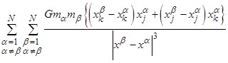
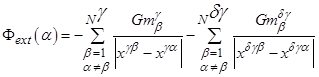
Now for the start, let us assume a set of N mutually gravitating particles / point masses in a system. Let the ath particle / point mass has mass Ma, and is in position x_a. In addition to the mutual gravitational force, there exists an external   f_ext, due to other systems, ensembles, aggregates, and conglomerations etc., which also influence the total force Fa acting on the particlea.  Here in this case, the f_ext is not a constant universal Gravitational field but it is the total vectorial sum of fields at x_a due to all the particles / point masses external to its system bodies and with that configuration at that moment of time, external to its system of N particles / point masses.

Total Mass of system =                                                                                      (1)

Total force on the particle a is Fa , Let Fab is the gravitational force on the a th particle / point mass due to bth particle.

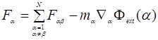                                                                                        (2)

Moment of inertia tensor

Consider a system of N particles / point masses with mass Ma, at positions Xa, a=1, 2,…N; The moment of inertia tensor is in external back ground field f _ext.

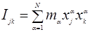                                                                                                                    (3)

Its second derivative is [Equation (4) removed]

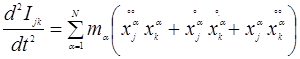                                                                 (4)

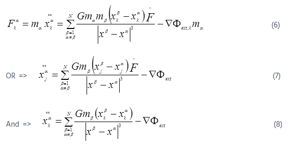
The total force acting on the particle a is and is the unit vector of force at that place of that component.

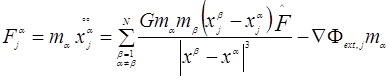                               (5)

Writing a similar formula for F^a_k 

Lets define Energy tensor ( in the external field  f_ext   )

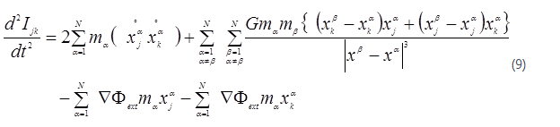(9)

Lets denote Potential energy tensor = Wjk =

                                                             (10)

Lets denote Kinetic energy tensor = 2 K_jk =                                         (11)

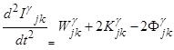
Lets denote External potential energy tensor = 2 F_jk

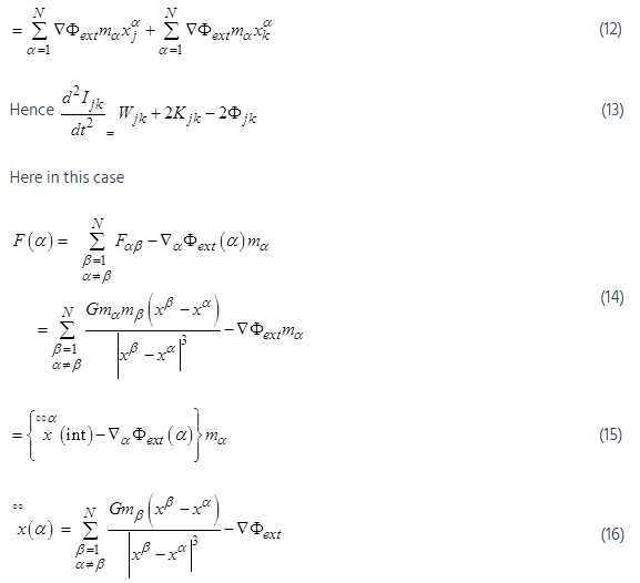
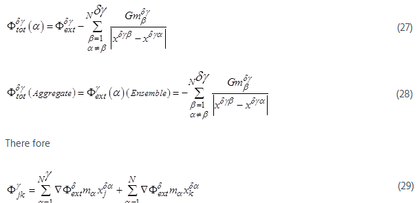
We know that the total force at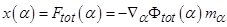

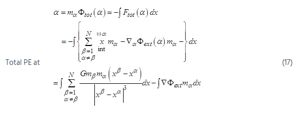
There fore total Gravitational potential f_tot (α)  at x (α) per unit mass

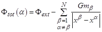                                                                                                 (18)

Lets Discuss the Properties of  f_ext :-

f_ext can be subdivided into 3 parts mainly

f_ext due to higher level system, f_ext -due to lower level system, f_ext due to present level. [ Level : when we are considering particles in the same system (Galaxy) it is same level, higher level is cluster of galaxies, and lower level is planets & asteroids].

f_ext due to lower levels : If the lower level is existing, at the lower level of the system under consideration, then its own level was considered by system equations. If this lower level exists anywhere outside of the system, centre of (mass) gravity outside systems (Galaxies) will act as unit its own internal lower level practically will be considered into calculations. Hence consideration of any lower level is not necessary.

System – Ensemble

Until now we have considered the system level equations and the meaning of f_ext . Now lets consider an ENSEMBLE of system consisting of N₁, N₂ … Nj particles in each. These systems are moving in the ensemble due to mutual gravitation between them. For example, each system is a Galaxy, and then ensemble represents a local group. Then number of Galaxies is j, Galaxies are systems with particles N1, N2 ….NJ, we will consider f_ext as discussed above. That is we will consider the effect of only higher level like external Galaxies as a whole, or external local groups as a whole.

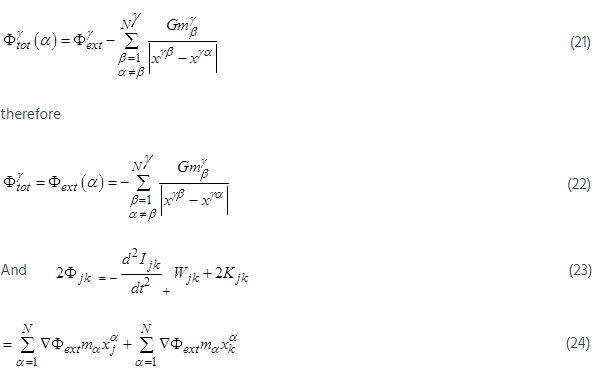
Ensemble Equations (Ensemble consists of many systems)

                                                                                                                (19)

Here ^γ  denotes Ensemble.

This F^γjk is the external field produced at system level. And for system

                                                                                                                    (20)

Assume ensemble in a isolated place. Gravitational potential  f_ext(a)produced at system level is produced by Ensemble and f^γ _ext(a) = 0 as ensemble is in a isolated place.

AGGREGATE Equations (Aggregate consists of many Ensembles )

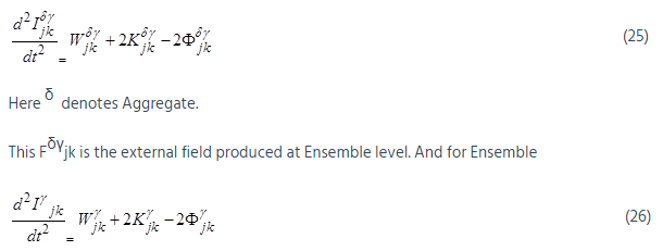
Assume Aggregate in an isolated place. Gravitational potential f_ext (a) produced at Ensemble level is produced by Aggregate and f ^δγ _ext(a) = 0 as Aggregate is in a isolated place.

And

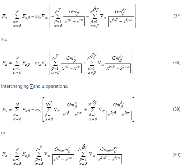
Total AGGREGATE Equations :( Aggregate consists of many Ensembles and systems)

Assuming these forces are conservative, we can find the resultant force by adding separate forces vectorially from equations (20) and (23).

                                                                           (30)

This concept can be extended to still higher levels in a similar way.

Corollary 1:

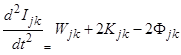                                                                                                                    (31)

 The above equation becomes scalar Virial theorem in the absence of external field, that is f=0 and in steady state, 

i.e                                                                                                                                                   (32)

        2K+ W = 0                                                                                                                                              (33)   

But when the N-bodies are moving under the influence of mutual gravitation without external field then only the above equation    (28)   is applicable.

Corollary 2:

Ensemble achieved a steady state, 

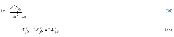
This  Fjk external field produced at system level. Ensemble achieved a steady state; means system also reached steady state. 

Combining both 3 and 25 (Newly introduced in this paper)

The above equation 35 means the force on α^th point mass will be a sum of three components i.e., the summation of attraction forces due to point masses from its own system, ensemble and aggregate. This is the key result that can be applied to point masses or subatomic particles or combined in any fashion together. The equations 34 & 35 are important, simple & straight forward results.

SITA: Blue Shifted Galaxies Graphs and Numerical Outputs& New Simulations

Resulting Graphs of Old Simulations for Blue Shifted Galaxies

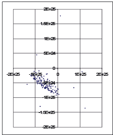
            From these resulting graphs one can see the orbit formations. When a uniform density of matter is assumed, say an equal point mass is placed in a uniform way in a three dimensional grid, all the point masses are collapsing into the CG of the set of masses. That means all are coming near and are Blue shifted. Orbit formations are happening only in non-uniform density distributions.

All the calculations were done using a small number of point masses. But the results were extremely encouraging. Always similar mass structures at large scale were formed in three dimensions showing lumpy formulations. Higher (super) computers can take up more number of point masses and show the empty nature of the formation to a greater detail in a faster manner.

Irrespective various starting positions of masses, the final stabilized mass positions are similar. The higher distance between the masses like great walls, the faster the movements are. The extremely distant galaxies are moving faster with huge red and blue shirts and with high velocities. The fallowing graphs are from the old 2004 paper. In this paper only typical pictures were presented.

Graph G1              :               Show initial random positions.

Graph G3              :               Shows picture after one time step, a lump formation was seen.

Graph G4            :           Now after two time steps the lump was stretched.  Lump was still stretched after 3 time steps and initial mass rotation formations are seen.

Graph G6              :               Randomly positioned masses started showing circular orbit formations

Graph G8              :               Orbit formations are clearer and all masses started following huge orbits depending on the masses.

There is no gravitational collapse of masses. Here there was no gravitational repulsion was present. All masses form orbits and move in orbits.

Graph: G1:

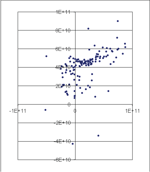
Graph G3 and G4

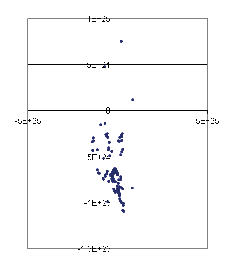
Graph  G6

Graph G8

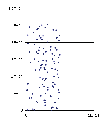
Graph: G1: Starting Pictures of xy Positions of Clusters (right) and Globular Clusters (left), x and y axes Scales Represent Distances in Meters. These Masses are Randomly on xyz axes. An Orbit Formation means some Galaxies are coming near (Blue shifted) and some are going away (Red Shifted.)

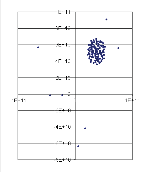
Graph G3 and G4 : G3 And G4 Represent the Positions of All Masses in this Simulation, After one Time-Step and Two Time-Steps. Here the Masses Hidden in the Graph G1 are Also Visible Which were Visible as a Small Dot Near the Zero of Xy Axes, and Which were Shown in Graph G1 in an More Elaborate Way. We Can See the Formation Of Some Three-Dimensional Circles Clearly

Graph  G6 : G6 represent the Positions of all Masses in this Simulation, after three and four time-steps. We can see the Formation of some Three-Dimensional Circles clearly

Graph G8: G8 represent the Positions of all Masses in this Simulation, after four time-steps and Seven Time-steps. We can see the formation of some three-Dimensional Circles clearly. That means Orbit Formation

Four New Simulations

New simulations were carried out on this subject. These are four more simulations with different kinds of input data. Four more files are being attached in Excel format which have all the output 3000 graphs and initial input data. Each is about 10 MB. In all these four simulations, all point masses have different distances and masses. The simulations are…

- All point masses are Galaxies

- All point masses are Globular Clusters

- Globular Clusters 34 Galaxies 33 aggregates 33 conglomerations 33

- Small star systems 10 Globular Clusters 100 Galaxies 8 aggregates 8 conglomerations 7

Rotations of Galaxies and orbit formations are visible in all types of formations.I will send any other data files upon further request.

Results of New Simulations

Rotations of Galaxies and orbit formations are visible in all types of formations.

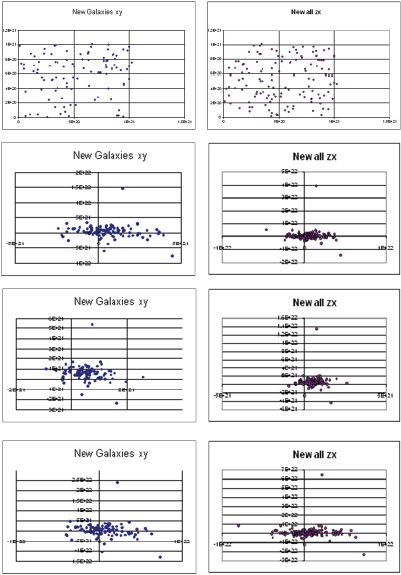
9.3 Graphs from‘all Point Masses are Clusters (approximately 10⁹ stars) ’ Simulation

In the above set of figures First column group of Graphs were with the name New Galaxies xy. Figures in the second column group of Graphs were with the name New all zx. These are XY and ZX plots of positions of Clusters approximately have the mass of about a billion or  10⁹ solar masses. First set is about 100 and second set is for all 133 Galaxies / clusters. All these are point masses for Galaxies but of smaller sizes.  The word ‘new’ in the name is an indicative word for the result of that particular iteration in the simulation. The first iteration is the starting positions of the Galaxies in xy or zx plots. From that with a time step of 3.15576E+15 seconds or 100 million years is allowed for the free fall of all the Galaxies. Next set of positions is shown in the iteration 1. After that is iteration 2 and so on. One can see the rotations of these masses. And the marked change of positions from iteration to iteration when we look through the series of graphs.

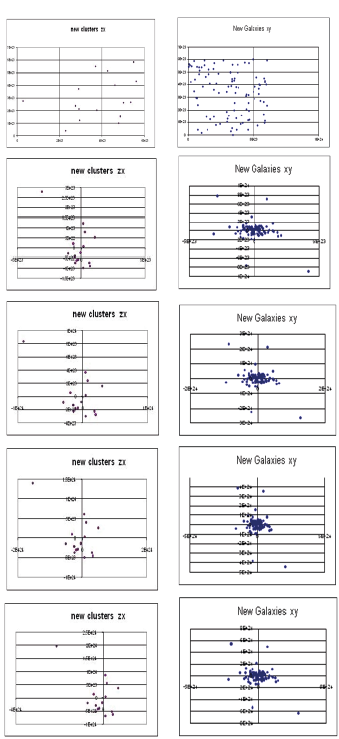
9.4 Graphs from ‘All Point Masses are Galaxy Ensembles’ Simulation

Here in this example (in this new simulation), in the above set of figures, the first column group of Graphs were with the name New Clusters zx. Figures in the second column group of Graphs were with the name New Galaxies xy. These are XY and ZX plots of positions of Clusters (or Galaxies) approximately have the mass of about a billion or 10¹² solar masses. First set is about 20 and second set is for all 100 Galaxies / clusters. All these are point masses for Galaxies of normal sizes.  The word ‘new’ in the name is an indicative word for the result of that particular iteration in the simulation. The first iteration is the starting positions of the Galaxies in xy or zx plots. From that with a time step of 3.15576E+15 seconds or 100 million years is allowed for the free fall of all the Galaxies. Next set of positions is shown in the iteration 1. After that is iteration 2 and so on. One can see the rotations of these masses. And the marked change of positions from iteration to iteration when we look through the series of graphs.

The set of graphs depicting the positions of all the point masses were omitted here due to space constraints. The change in positions is visible only in the first few graphs for all the point mass positions.

The ‘New clusters zx’ graphs indicate a subset of all Galaxies is rotating about. These graphs will show the observer, some Galaxies are coming near and some are going away. Hence these galaxies are either red shifted or blue shifted.

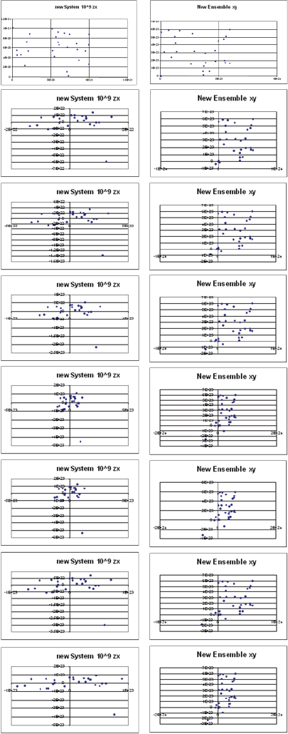
9.5 Graphs from ‘Globular Clusters 34 Galaxies 33 Aggregates 33 Conglomerations 33’ Simulation

Here in this example (in this new simulation), in the above set of figures, the first column group of Graphs were with the name New System 10^9 zx. Figures in the second column group of Graphs were with the name New Ensembles xy. These are XY and ZX plots of positions of Globular Clusters and Galaxies approximately have the mass of about 100 million to a billion or 10¹² solar masses. First set is about 34 and second set is for all 33 Galaxies. All these are point masses for Galaxies of normal sizes.  The word ‘new’ in the name is an indicative word for the result of that particular iteration in the simulation. The first iteration is the starting positions of the Galaxies in xy or zx plots. From that with a time step of 3.15576E+16 seconds or one billion years is allowed for the free fall of all the Galaxies. Next set of positions is shown in the iteration 1. After that is iteration 2 and so on. One can see the rotations of these masses. And the marked change of positions from iteration to iteration when we look through the series of graphs.

The set of graphs depicting the positions of all the point masses were omitted here due to space constraints. The change in positions is visible only in the first few graphs for all the point mass position graphs.

These two columns of graphs indicate all Galaxies are rotating about. These graphs show to the observer, some Galaxies are coming near and some are going away. Hence these galaxies are either red shifted or blue shifted.

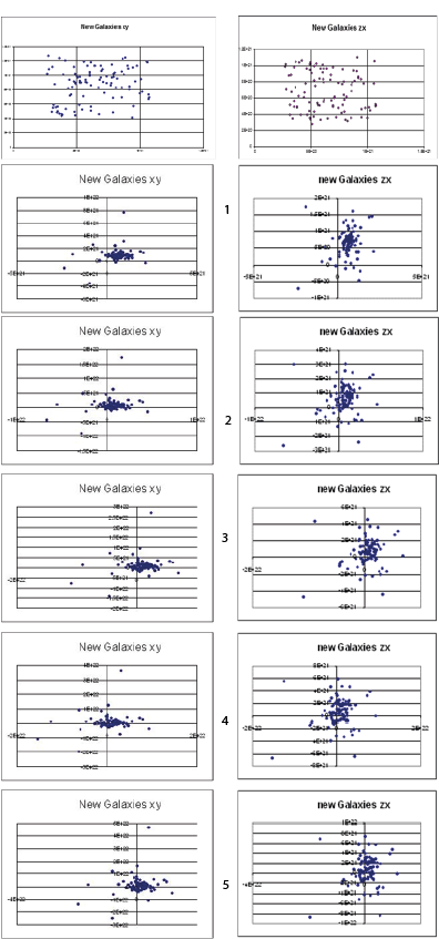
9.6 Graphs from ‘Small Star Systems 10 Globular Clusters 100 Galaxies 8 Aggregates 8 Conglomerations 7’ Simulation

Here in this fourth example (in this new simulation), in the above set of figures, the first column group of Graphs were with the name New Galaxies xy. Figures in the second column group of Graphs were with the name New Galaxies zx. These are XY and ZX plots of positions of 100 Galaxies approximately have the mass of about a billion or 10¹² solar masses.

Here xy and zx plots of the same 3 dimensional point mass positions were chosen so that one can imagine the three dimensional picture of the same set. These graphs represent the output of SITA simulations for the same iteration and for the same set of masses.

All these are point masses for Galaxies of normal sizes.  The word ‘new’ in the name is an indicative word for the result of that particular iteration in the simulation. The first iteration is the starting positions of the Galaxies in xy or zx plots. From that with a time step of 3.15576E+15 seconds or one billion years is allowed for the free fall of all the Galaxies. Next set of positions is shown in the iteration 1. After that is iteration 2 and so on. One can see the rotations of these masses. And the marked change of positions from iteration to iteration when we look through the series of graphs.

The set of graphs depicting the positions of all the point masses, all other different varieties of masses  were omitted here due to space constraints. The change in positions is visible only in the first few graphs for all the point mass position graphs.

These two columns of graphs indicate all Galaxies are rotating about. These graphs show to the observer, some Galaxies are coming near and some are going away. Hence these galaxies are either red shifted or blue shifted.

Discussion

In this model both red shift and blue shift of galaxies are possible simultaneously in all directions and at all distances from us. That depends only on location of distant rotating and revolving cluster.

We can say that:

1. The RATIO Blue to Red shifted galaxies will never be 50:50
2. The galaxies that appear to come near (Blue Shifted) will always present in the total number of galaxies. This number is not zero as predicted by expanding universe models.
3. The percentage of blue shifted galaxies will vary from place to place. That depends on many factors, like the FORMATION OF IMAGES IN THAT AREA. Images may be formed for the whole of local group itself.
4. The number of blue shifted Galaxies depend on the orientation of the planar revolving cluster of galaxies with respect us.
5. We will assume Hubble law for empirical distances of galaxies as   v = cz = H_oD. Where v is the velocity of the galaxy, c is the velocity of light, z is the red shift, D is the distance of galaxy, H_o is the Hubble constant for distance only not for expansion of universe.

The galaxies that appear to come near (Blue Shifted) will always present in the total number of galaxies. This number is not zero as predicted by expanding universe models. The percentage of blue shifted galaxies will vary from place to place. That depends on many factors, like the formation of images in that area. Images may be formed for the whole of local group itself. The number of blue shifted Galaxies depends on the orientation of the plane of revolving cluster of galaxies with respect us. For obtaining the real map of Universe, we have to eliminate all the images from the Map, for which a detailed probing of all Galaxies is required.

Conclusion

Hence we may conclude:

The actual ratio of Red shifted to Blue shifted Galaxies will depend on

a. Universal Gravitational Force acting on each Galaxy at that instant of time,

b. The position of the observer in the Universe

c. The actual point mass distribution in the universe in three dimensions at that instant of time. This ratio can never be 50:50.

Dynamic Universe model is based on hard observed facts and gives many verifiable facts.   In this paper the simulations predicted the existence of the large number of Blue shifted Galaxies, in an expanding universe, in 2004 itself. It was confirmed by Hubble Space Telescope (HST) observations in the year 2009. This prediction process is clearly shown the output pictures formed from this Model from old and new simulations. These pictures depict the three dimensional orbit formations. An orbit formation means some Galaxies are coming near (Blue shifted) and some are going away (Red shifted). This paper goes on two main lines. First is the main line of thinking, to show mathematically that there will be lots and lots of blue shifted Galaxies. To support this concept the question what are the possible blue shifted Galaxies is answered further. We find that quasars are blue shifted galaxies. The second line of thinking goes with this finding, that the Quasars are blue shifted galaxies. Now it can be 32% of total Galaxies are blue shifted in this universe.

Acknowledgements

I sincerely thank Maa Vak for continuously guiding this research.

References

1. Rubin VC (2000) One Hundred Years of Rotating Galaxies. Publications of the Astronomical Society of the Pacific 112: 747–750. [crossref]
2. Rubin VC (1983) Dark matter in spiral galaxies SciAm  248: 96–106. [crossref]
3. Narlikar JV (1983) Introduction to cosmology.  Foundation books, New Delhi , India.[crossref]
4. Tully RB, Fisher JR (1987) Nearby Galaxies Atlas. Cambridge University Press, Cambridge, England. [crossref]
5. Tipler FJ (1996) Newtonian cosmology revisited. Monthly Notices of Royal Astronomical Society 282: 206–210.  [crossref]
6. Shi X, Turner MS (1998) Expectations for the difference between local and global measurements of the Hubble constant. Astrophys J 493: 519–522. [crossref]
7. Aguirre A ,Gratton S (2002) Steady-State Eternal Inflation. Phys Rev 65. [crossref]
8. S.N.P. GUPTA (2015) No Dark Matter’ Prediction from Dynamic Universe Model Came True!. JAAT 3. [crossref]
9. S.N.P.GUPTA (2010) Dynamic Universe Model: A singularity-free N-body problem solution. VDM Publications, Saarbrucken, Germany. [crossref]
10. S.N.P.GUPTA (2011) Dynamic Universe Model: SITA singularity free software. VDM Publications, Saarbrucken, Germany. [crossref]
11. S.N.P.GUPTA (2011) Dynamic Universe Model: SITA software simplified. VDM Publications, Saarbrucken, Germany. [crossref]
12. S.N.P.GUPTA, Murty JVS, Krishna SSV (2014) Mathematics of dynamic universe model explain pioneer anomaly, Nonlinear Studies. USA 21: 26-42. [crossref]
13. S.N.P. GUPTA (2013) Introduction to Dynamic Universe Model. IJRR  2: 203-226. [crossref]
14. Einstein A (1952) The foundation of the general theory of relativity". In H.A. Lorentz, A. Einstein, Minkowski H and Weyl H The Principle of Relativity: A Collecton of Original Memoirs on the Special and General Theory of Relativity, with Notes by A. Sommerfeld. Dover, USA 109-164. [crossref]
15. S.N.P.GUPTA (2014) Dynamic Universe Model’s Prediction No Dark Matter in the Universe Came True!. Appl Phys Res  6: 8-25. [crossref]
16. S.N.P.GUPTA, Dynamic Universe Model Predicts the Live Trajectory of New Horizons Satellite Going To Pluto. Appl Phys Res  7: 63-77. [crossref]
17. S.N.P.GUPTA (2014) Dynamic Universe Model Explains the Variations of Gravitational Deflection Observations of Very-Long-Baseline Interferometry. Appl Phys Res 6: 1-16. [crossref]
18. Obukhov YN (1992) Rotation in Cosmology.  General Relativity and Gravitation 24: 121-128. [crossref]
19. Carneiro S (2000) A Gödel-Friedmann cosmology?. Phys Rev 61. [crossref]